Artificial Neural Networks

Have you ever used something having no clue of how it works?

You’re not alone!

This post aims to demystify a bit the processes going under a neural network model and explain how it is composed internally.

Motivation

When I just started getting familiar with neural nets, I was reading hundreds of articles that were full of math, starting from simple operations with matrices and finishing with partial derivatives and complex functions.

Yeah, and probably the most exciting question is how I didn’t get bored while reading all this theoretical stuff. Well, the answer is simple.

I get very, very, very bored!

But still, after a huge number of complex math articles and white nights, I didn’t have a complete understanding of what a Neural Net model is.

Now I have a way more clear vision about how all this stuff works internally and writing this post I hope that it will help to make things more clear for you as well.

Where to Start?

Well, the first thing that I figured out is that a Neural Network is not the most suitable name for a mathematical model because it’s already reserved for the real biological one from human being’s brains and would be more accurate to call it Artificial Neural Network or ANN instead.

So knowing this, it’s already clear that Artificial Neural Network(ANN) is nothing else than a mathematical model of a real biological Neural Net.

And here I finally released that I was trying to learn how to build a math model of something that I didn’t know how it works.

Yes, you got me, right! And probably it sounds apparent to you, but it would be much easier to build a math model of a Neural Net when you know how it works.

That’s why I decided to study Neural Nets from the biological point of view first and then came back to math.

Real Neural Networks

And here I want to congratulate you being one of the least people not scared by biology and who continued reading this post. Hurry to let you know that we’ll not dive too deep into biology stuff, but still, you should remember at least the high school biology classes. So let’s get started!

The role of a biological neural net is to take some information in the form of some electrical signals and generate an output by propagating those signals through its neurons.

But what is a neuron?

Neuron, also known as a nerve cell, is an electrically excitable cell which receives, processes, and transmits information through electrical and chemical signals and which is composed of 4 main parts:

1. Dendritic Tree
2. Cell Body
3. Axon
4. Synapse

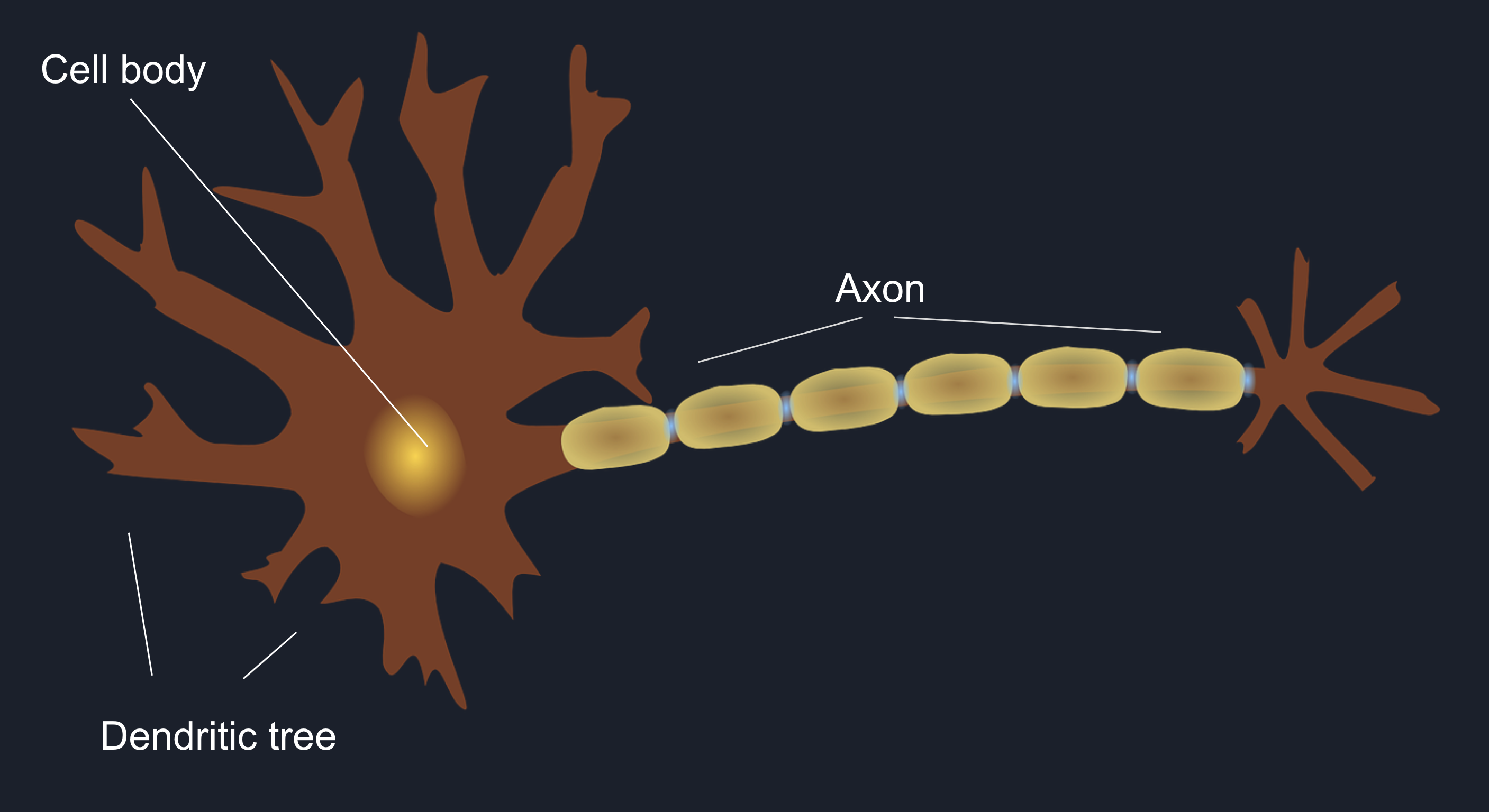
It receives some signals from other neurons through its dendritic tree, which are being collected, summed up, and transported to the hillock. In case the accumulated signal is large enough, it will trigger an action potential on the axon, causing the signal to travel down the axon’s bounds right to the next neuron.

Ok, the above definition explains how the signal travels through a neuron cell starting from its dendrites and finishing with axonal terminals, but how it reaches the next neuron?

So, as said before, neurons are connected into a network. This happens through special connections called synapses.

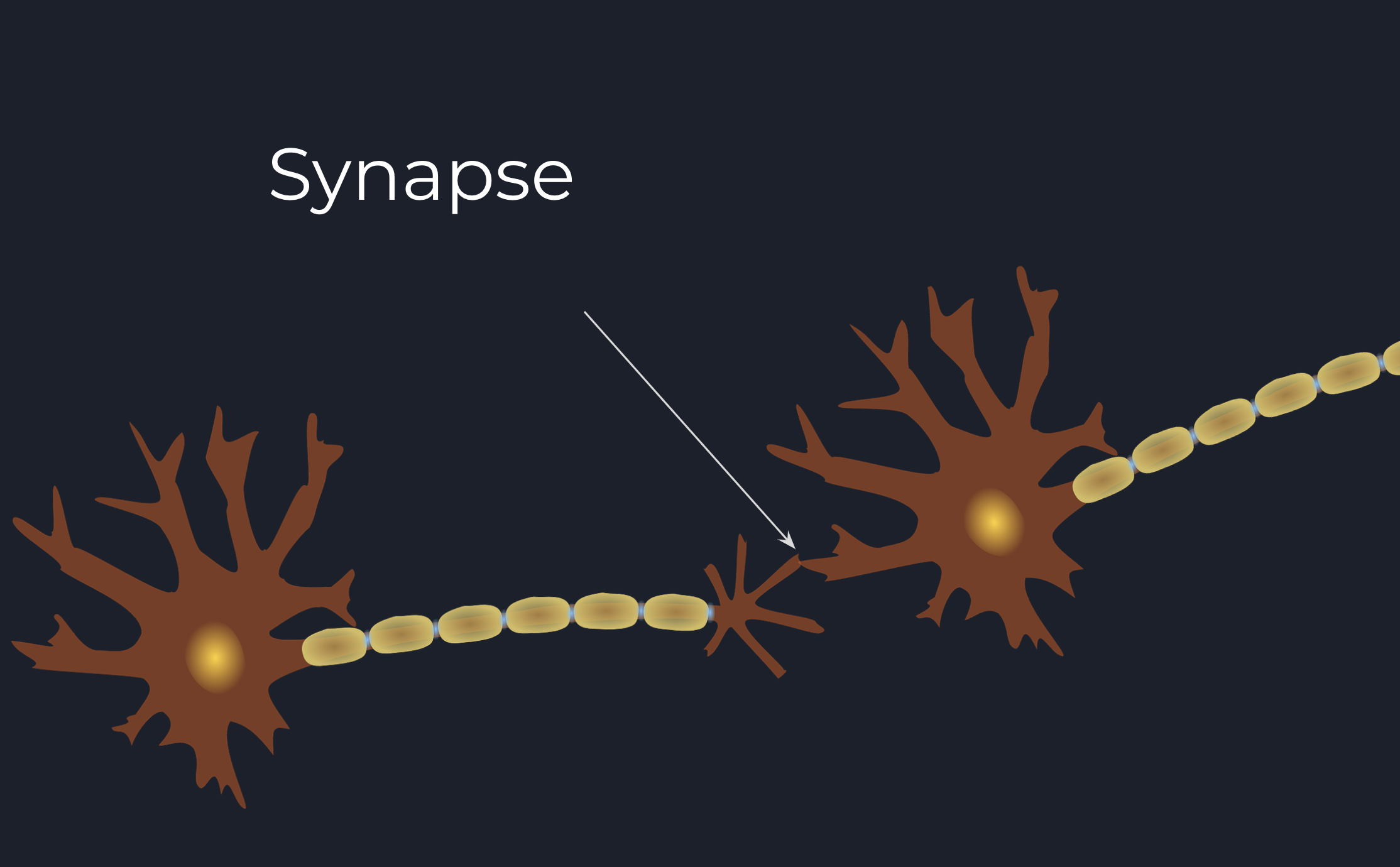
Basically, a neuron becomes connected to another neuron when at least one of its axonal terminations is extremely close to one of the dendrites of that neuron to form a Synapse. A synapse is a small biological junction; a neuron signal can be sent through.

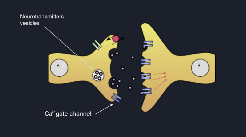
The most interesting part is that the neurons are incredibly close, but not touching each other. There is a small space between their membranes called Synaptic Cleft.

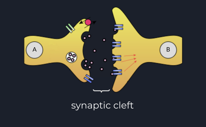
When we have 2 neurons connected through a synapse, and the first neuron fires, which means that there was enough accumulated signal at its hillock, the voltage potential across the membrane is positive enough to trigger some sodium channels close to axonal terminals open. This allows a fluid of sodium to penetrate the cell and trigger another Ca²⁺ channel open and allow Ca²⁺ flow inside the axonal termination.

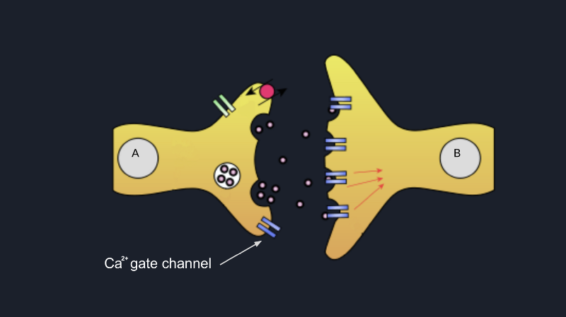
Most probably, you know that in any axonal termination, there exist some vesicles that act as kind of containers for some molecules called neurotransmitters (serotonin, dopamine, epinephrine) and which are docked to the pre-synaptic neuron’s membrane by some special proteins called SNARE proteins.

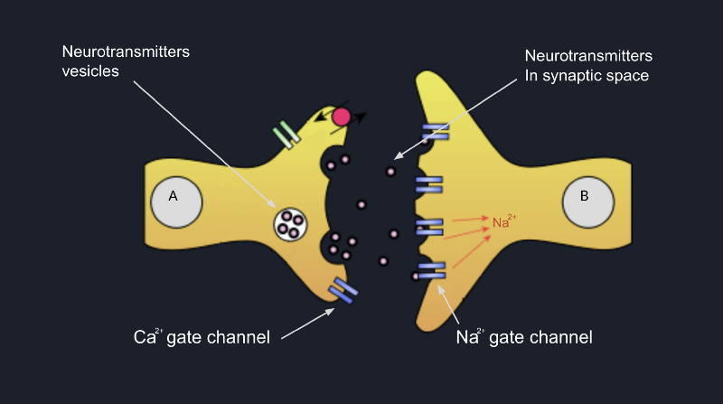
When Ca²⁺ ions get inside the axonal termination, it changes the configuration of the SNARE proteins enough to make them bring the vesicles with neurotransmitters as close as possible to the membrane such as in the end their membranes merge, and all neurotransmitters are dumped into the synaptic cleft as shown in the picture below.

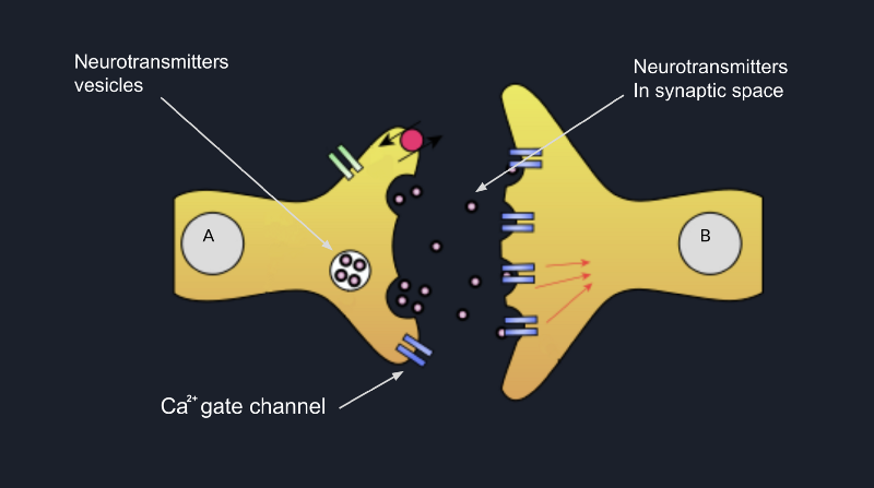
This process is called exocytosis. Consequently, all these neurotransmitters being in the synaptic cleft, they bound to the membrane of the postsynaptic neuron, which can trigger some sodium channels open and allow Na²⁺ flow inside the cell. This way, the dendrite of the postsynaptic neuron will be excited, and most probably if some other dendrites of this neuron will also be excited by some other neurons, and the cell will accumulate enough positive potential, the neuron will fire, and the signal will go forward to the next neuron.

Are you filling confused a bit?

Don’t worry about this! Just imagine how much I was, reading all this stuff myself trying to figure out the connection between math and biology. I will do a small recap in the next chapter to make everything more straightforward for you. You can also re-read this section, and I bet you’ll understand it better.

Artificial Neuron (Back to Math!)

Glad to see you reached this part of the post, we are going to do some math soon but before we start, as we are going to model mathematically the stuff that we talked about above, let’s do a short recap and take a look at the steps one neuron passes a signal to another one:

1. The neuron will receive some signals through synapses from other neurons to some of its dendrites;
2. All these signals will be accumulated and summed up inside its cell body;
3. If the accumulated potential reaches a specific bound, a spike or a signal will go through the axon right forward to the axonal terminations to be consumed by the next neuron.

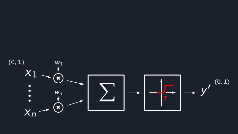
Now let’s try to create our very first artificial neuron by modeling the steps mentioned above.

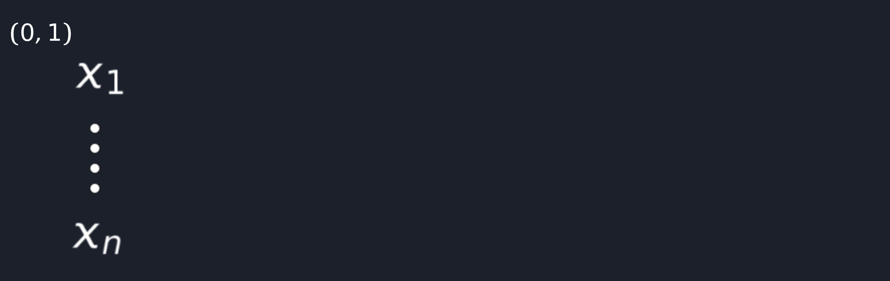
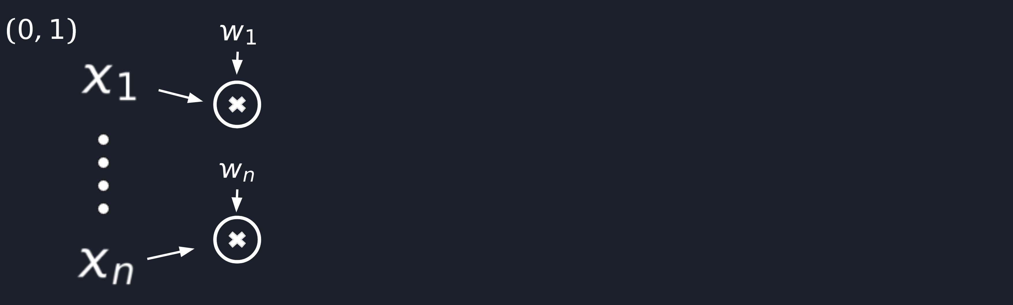
First of all, the neuron should receive some signals which we are going to represent as variables from X₁ to Xn, and for simplicity, let’s assume that they will take floating-point values from [0..1] range.

Step 1

All signals mentioned above should pass through synapses, right? We can achieve the same effect in math by multiplying each of our inputs by a W(weight), a predefined constant that will increase or decrease the input signal’s influence on the final result.

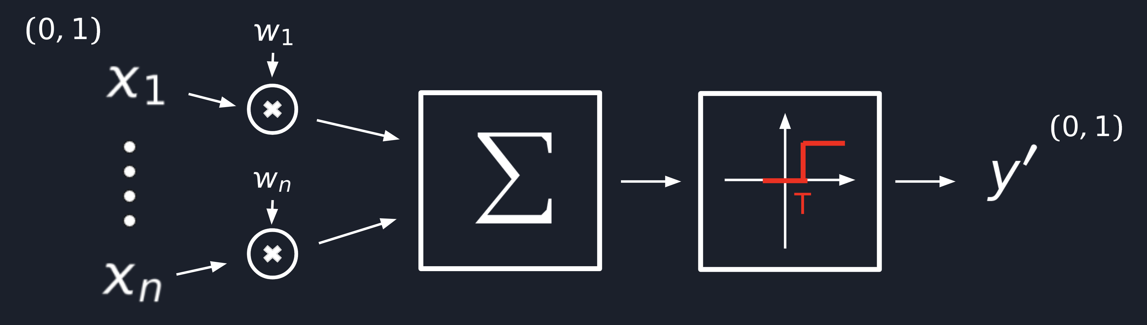
Step 2

I would say that this is the most obvious step which doesn’t need an explanation but still. We need to model the cumulative effect of the signal, and it’s clear enough that we’re going to do this by adding a sum operator. (Hope you remember the notation from High School math classes.)

<img alt=”Neural Model step 2”src=”/assets/images/posts/neural-networks/neural-model-step2.png” />

Step 3

In the last step, we need to model somehow the effect of “fairing at some point” when there is enough signal accumulated. This can be done by introducing a simple step function. When the accrued signal reaches a specific T(threshold), we want to make the neuron fair, so that its output Y′ will be 1, which means the signal will be propagated forward and 0 in other cases.

Congratulations!

We finally defined an artificial neuron which:

1. Gets some input [X₁..Xn] through its Synapses(multipliers) or W(weights)
2. Accumulates it in its cell body(the sum operator)
3. And fires in case the quantity of accumulated signal reaches a specific T(threshold)

Now, most probably, you’re asking yourself why we didn’t reach the terminator epic like scenes yet, right?

Well, the answer is simple. There are a lot of factors we cannot model mathematically because we don’t know how they work from the biological point of view yet, like:

1. Refractory rate;
2. Axonal bifurcations;
3. Time patterns.

etc.

Artificial Neural Network (ANN)

Now when we got an idea of how a Biological Neural Network works and how we can model it mathematically, let’s do it!

To smooth our transition from different pictures and diagrams to math formulas we might imagine a neural network in a more simplified form as a box full of W(weights) and T(thresholds) in which comes in a variety of inputs from X₁ to Xn and comes out a set of outputs let’s say from Y′₁ to Y′n as shown in the picture below.

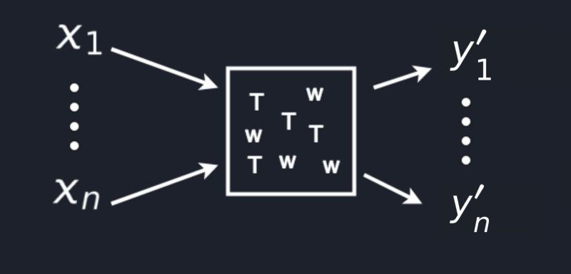
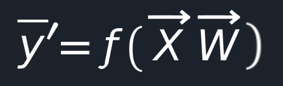
Now, all this stuff can be converted extremely nice to a mathematical function that you can use for predictions later on.

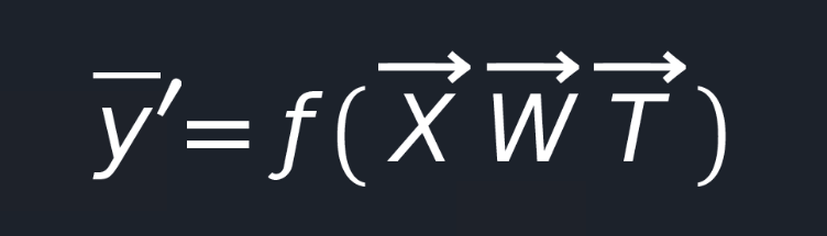
Let’s abstract a bit from a real implementation and see how we can use this function. Suppose we want to build a neural network able to recognize handwritten digits. We’ve got our function, we have an input X which is a picture of a handwritten digit, we apply our function and get an output Y′ which should be the number recognized from the picture.

But wait! What values should take W and T?

Well, we have already mentioned that W(weights) and T(thresholds) are some predefined constants. We just need to find the most suitable values for them such that when we have an input value X, we’ll get a desired, close to real, predicted output value for Y′.

You’re probably asking yourself how the hell I can find the correct values for T and W. Well, this process is called Training, and it is one of the most complicated topics in the massive universe of ANN.

Yes! You have an Artificial Neural Net(a brain), and you have to train it before use. That’s freaking awesome, isn’t it?

So let me start with T(thresholds). The easiest way to find a suitable variable for them is to not do this. We can easily get rid of them by following these 3 simple steps:

1. Assume that one weight let’s say W₀ equal T(threshold);
2. Connect an input X₀ which will always equal -1;
3. This means that we’ll obtain -T because our input X₀ passing the synapse will get multiplied by our weight W₀. The -T value will be summed up with all other results and will move our threshold value to the origin.

Now our neural net function looks way simpler, and we left to find a suitable value for our W(weights).

But how can we do it?

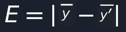
Given that Y′ is the output from our function and let Y be the desired output, we can easily define an error function, can’t we?

Using this, we can see how well our neural net is performing. Now our task is to choose such a value for W(weights) so that the E(error) will be as close as possible to 0.

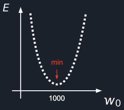
Most probably, if you’re a programmer, you’ll have the same idea I had.

Lets brute force it!

To do this, we just need to write a program which will take different values one by one for W(weight) and will compute the E(error) so that in the end, we just pick up the W(weight) which gave us the smallest E(error).

Done!

But wait! It’s too easy to be real, isn’t it?

Yeah, it’s not a suitable solution for us. Let’s see why:

At the first look, this task is straightforward and can be executed in a few ms even by our personal computers. But this is just in case we have only one W(weight). Unfortunately, it will take hours for just 3 W(weights), and years of computation in case we try to do it for 9 W(weights).

I am sure you don’t want a neural network that will spend years learning something to answer 42 in the end.

Yeah, but can we optimize our computations?

Yes! Another solution would be to:

1. Take a random value for our W;
2. Take a value from the left of our current W and the right;
3. Compute error for those values and see in which direction the error decreases;
4. And then just go in that direction and repeat the same process again.

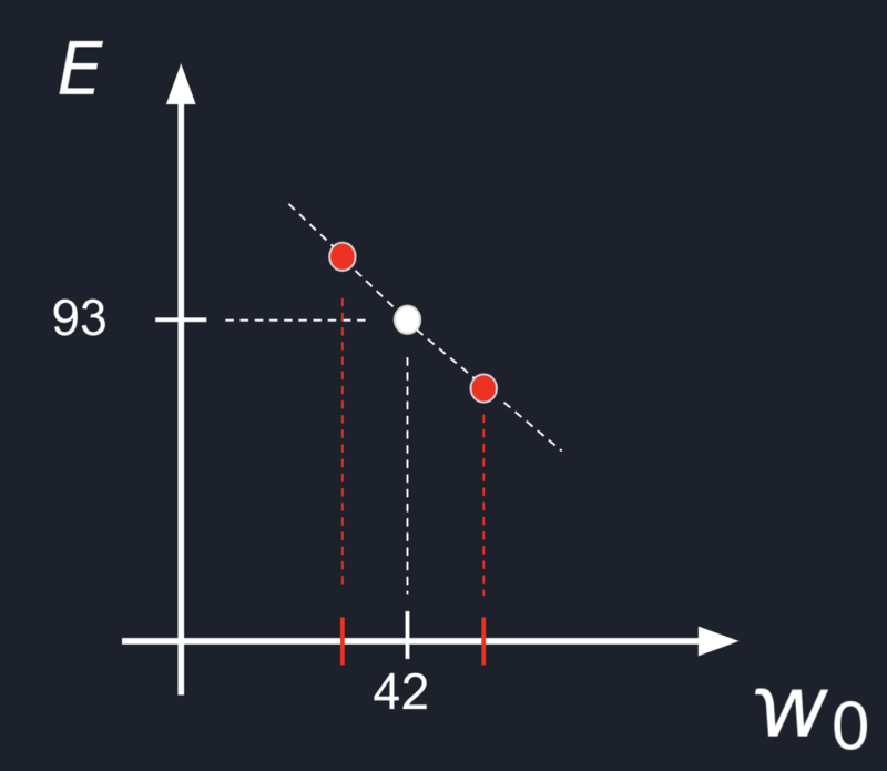
This approach is called Numerical Gradient Approximation, and it will optimize our computations by excluding several redundant operations.

But still, this is not the best we can do!

Let’s come back to our Neural Net error function for a moment.

We can easily replace Y′ in this equation and obtain this:

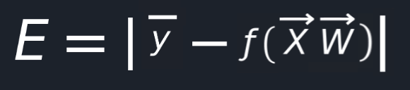
Now, we can compute the partial derivative of our E(error) function with respect to our W(weight) and find the exact direction in which our error will decrease.

This technique is called gradient descent, and it should optimize our computation a lot, but there is a small problem, we cannot use it yet! We cannot use it because we have a discontinuous function.

Do you remember our step function?

And actually, this had been a problem for around 25 years till Paul Werbos solved it in 1974 in his dissertation, which described the process of training artificial neural networks through backpropagation of errors for the first time. He replaced the step function with a sigmoid one.

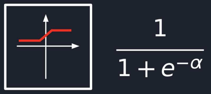
Well, the sigmoid function is convenient from different points of view, but the most important one is that it’s continuous, which allows us to easily apply the gradient descent technique!

But before going into back-propagation and gradient descent too deep, let’s try to build our first smallest artificial neural network in the world.

Smallest ANN in the World!

To build the smallest artificial neural network in the world, we need to build 2 artificial neurons and connect them. Let’s do it step by step:

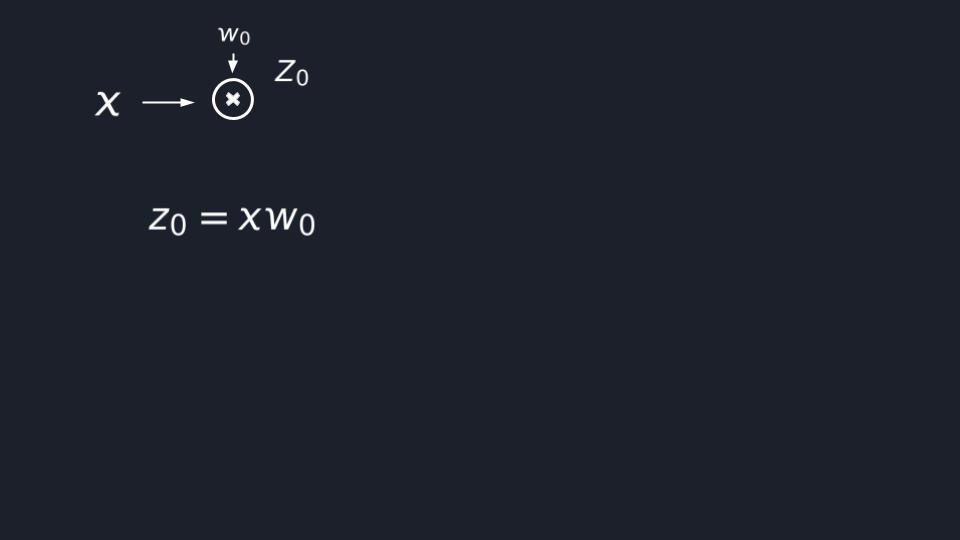
Step 1

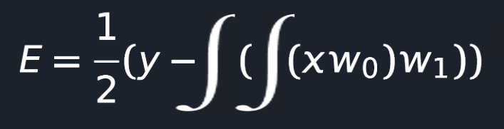
We’ve got our input variable X, and we need to multiply it with the W(weight) of the first neuron, right? So, we multiply X by W₀, and let’s store the result of this product into Z₀, where 0 is the index of the neuron.

Step 2

Now, the signal should go through a sigmoid activation function. I am going to notate it with this integralish sign just for simplicity. So in this step, we take the output from the previous one and apply the sigmoid function on it. And yes, let’s store it into α₀.

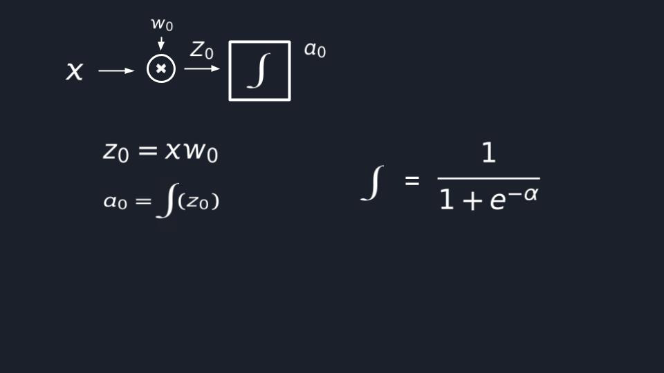
And here we’re done with the first neuron!

I bet you’re asking yourself where the hell the summation step is. Well, the answer is straightforward. We took a simple neural network example in which we have just one input X, so we don’t have what to sum up. ¯_(ツ)_/¯

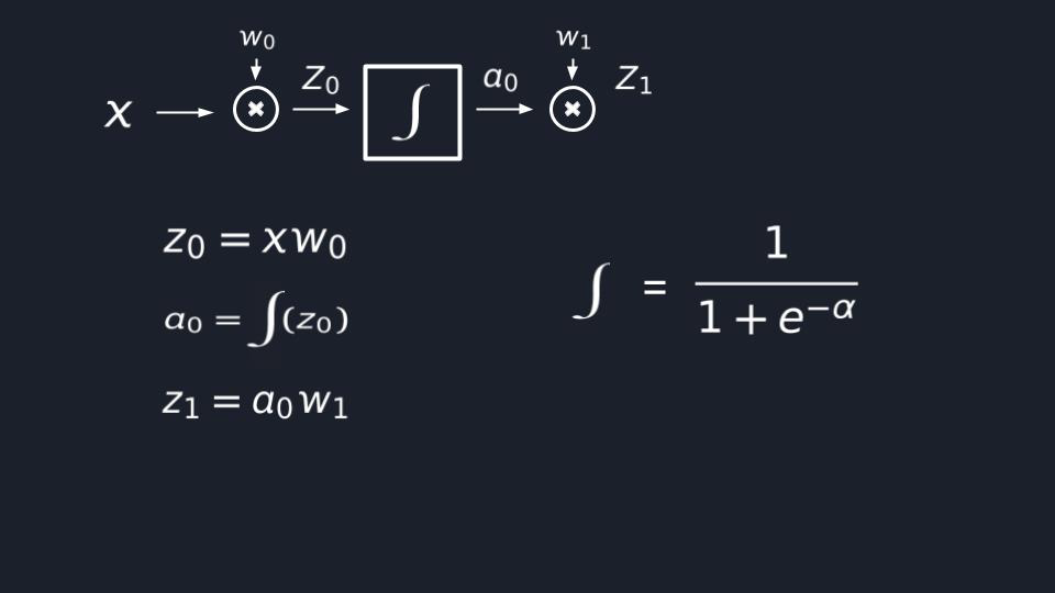
Step 3

In this step, we are going to propagate our signal to the next neuron. Thus, we just take the output of the previous step α₀, which is the output of the first neuron, and serve it as input for the second one by multiplying it with its W₁ and let’s also store this value to Z₁.

Step 4

And the last step is about applying the sigmoid function again but just other Z₁ in this case.

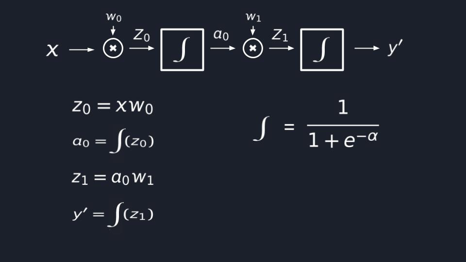
Done!

We have the smallest neural network in the world composed of 2 connected artificial neurons.

I hope you have already noticed that we can connect all formulas into one and obtain a single formula with one input variable X and 2 W parameters.

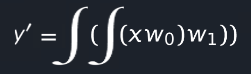
Yes! An ANN finally comes to be nothing else than a big universal function approximator with input variables and preconfigured W parameters.

Now let’s see how to apply gradient descent to train it to do something useful for us. :smily:

As I said before, we can generate an error function for our neural net, which will tell us how good it’s performing.

But, you know? We can improve it a bit.

1. We can remove the modulo in case we square it;
2. Also, multiplying it by 1/2 will be very handy later on.

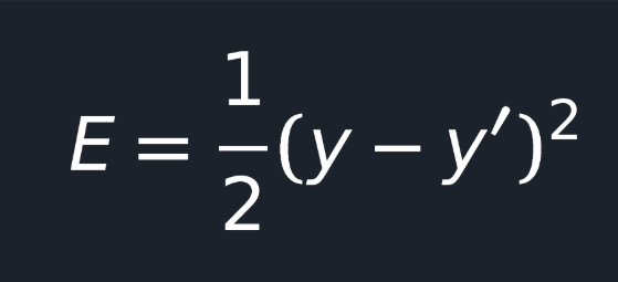
Sorry, but I don’t want to go into too many details here because choosing the correct error or cost function is a separate, vast, and complicated topic. There are a lot of error functions; however, in this case, we’re going to use MSE.

Now let’s replace our neural network function into the error one.

So, we need to adjust our weights in such a way that when we input a value for X the E would be as close as possible to 0. And as I told you before, we can’t apply brute force nor gradient numerical approximation as they will take too much computation time, and we’ll become old 👴 till our neural net will be trained.

What would save us in this situation is knowing the exact direction(decrease/increase) towards to change W₀ and W₁ such that our E will start moving to 0.

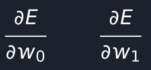
Thus, the solution is to compute the gradient!

We need to compute the partial derivative of the error with respect to W₀ and W₁.

I am not going to dive into too many details about Back Propagation in this post because I am planning a separate post on this topic special for freaking curious people like me.

In this post, I’ll just share already computed formulas given some small hints.

So, First of all, we have composed functions, so we need to apply the chain rule to compute the partial derivates.

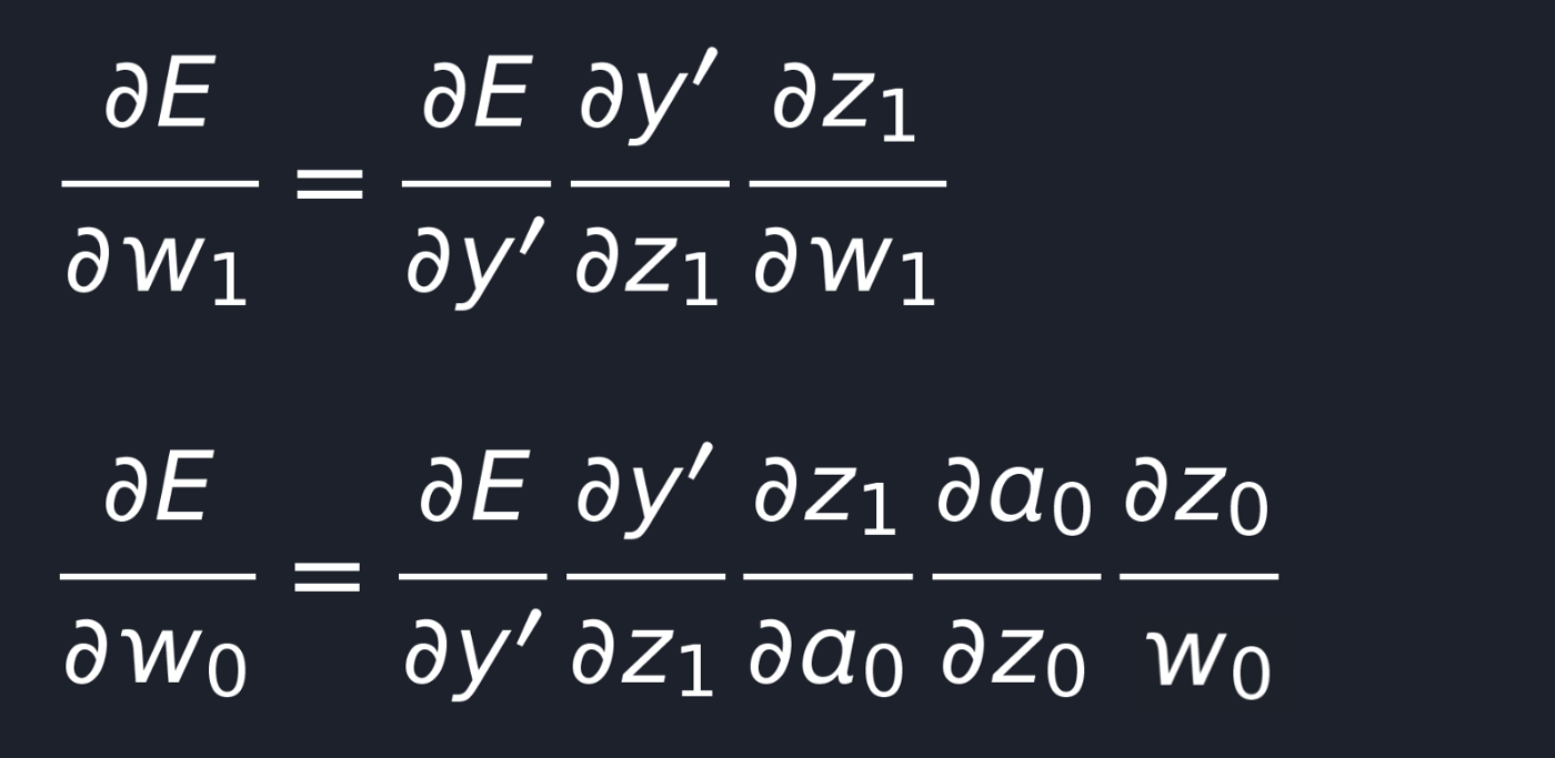
And if we compute the partial derivative for each term, we obtain the formulas below.

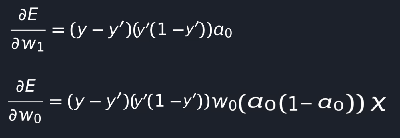
Now what’s left is just to replace variables with real numbers for an actual neural net with processing on real data, compute partial derivatives(the direction in which we need to update our weights), and using this, adjust the weights.

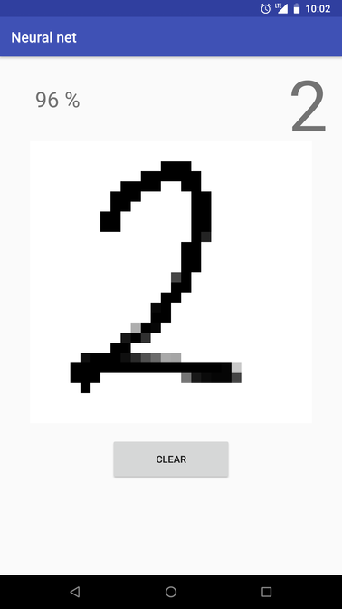
Stay tuned and wait for my next Handwritten Digits Recognition post to check out how to apply all this knowledge in practice and build a nice Android application able to recognize handwritten digits, as shown in the picture below.

Conclusion

So, to conclude, an Artificial Neural Network is nothing else than a mathematical model of a real biological Neural Network from our brains.

Almost everything around us could be described and modeled using math and functions, while AAN represents a function approximator. Thus, you basically compose a complex AAN function and then adjust its parameters so that the function itself will be as close as possible to the real one, and will start giving desired, close to real, predicted output values.

Of course, everything mentioned in this post is just the simplest part of the huge Machine Learning universe, but I believe it makes at least a clear vision of what basically ANNs are and how do they work.